Pure Lists with O(log(i)) Indexing
Linked lists are simple and ubiquitous. When used as a stack, they allow for constant time pushing and popping. Furthermore, they are purely functional: multiple processes can branch off of a linked list and push their own items without stepping on eachothers’ toes, so long as they avoid mutating the list. However, indexing into a list is slow: retrieving the i’th element of a list requires i “hops” along the items. While indexing isn’t technically required of a stack, it is often desired. (For example, when implementing an interpreter with De Bruijn indices, variable lookup requires indexing into the stack representing the environment.) As the title suggests, it turns out that we can improve upon lists to achieve O(log(i)) indexing without forfeiting purity and O(1) push/pop. I call them rainbow lists.
We take an approach similar to indexable skiplists and add shortcuts to each node of the list. However, while skiplists add an unbounded number of shortcuts per index and support insertion/deletion, we will add exactly 4 shortcuts and forego these operations, ultimately allowing us to maintain constant time push/pop. Okasaki’s skew binary random-access lists actually accomplish all of our goals and support updating, with only a minor hiccup. When indexing by i into a length n list, Okasaki’s lists take O(min{i, log(n)}) in the worst case and O(log(i)) in the expected case. Rainbow lists take exactly O(log(i)) which is barely an improvement. However, I find this approach elegant so I’d like to share it nonetheless. A Python implementation can be found at the bottom of this post.
The first type of shortcut we might wish to add to each node might be to skip ahead by 2^k indices, where 2^k is the largest power of 2 that divides i, the index of the node in the list. Recall that this 2^k can be computed in constant time as i & -i. This will give a nice mix of different range shortcuts and is suggestive of some sort of binary tree structure. I call these green shortcuts. We can depict the resulting data structure as below by drawing a green arc from every i to i-(i & -i) and a black arc from every i to i-1. Note that every arc goes from a larger index to a smaller one so I omit arrow heads.
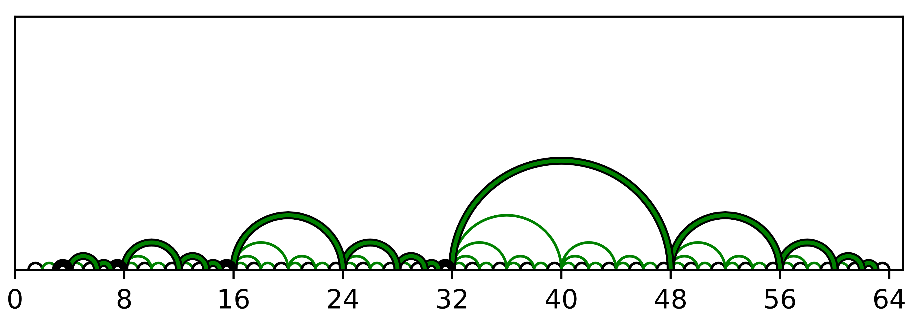
The above image highlights a path through green shortcuts and black next pointers from a node indexed 63 to one indexed 3. Computing a path in this case is simple because the arcs don’t cross so we can use a greedy algorithm: take a green shortcut unless it overshoots the target, in which case fall back to black. While this is already a massive improvement with very cheap data overhead, it doesn’t quite meet our goal. As can be seen in the image, this yields paths with log-many sequences of log-many green shortcuts, yielding log(i)² running time. This may be good enough for some applications where i tends to be quite small, but let’s press on towards our goal.
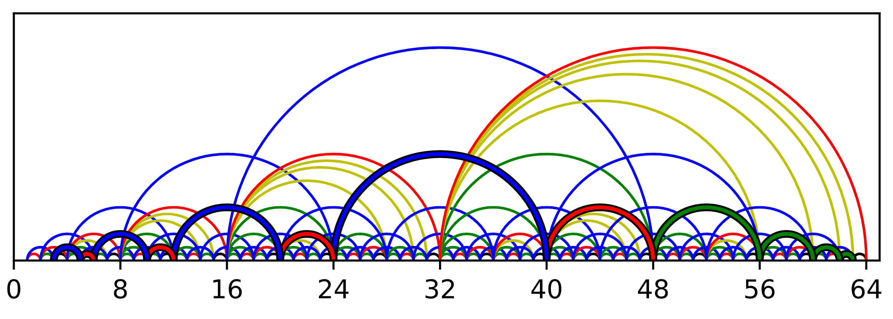
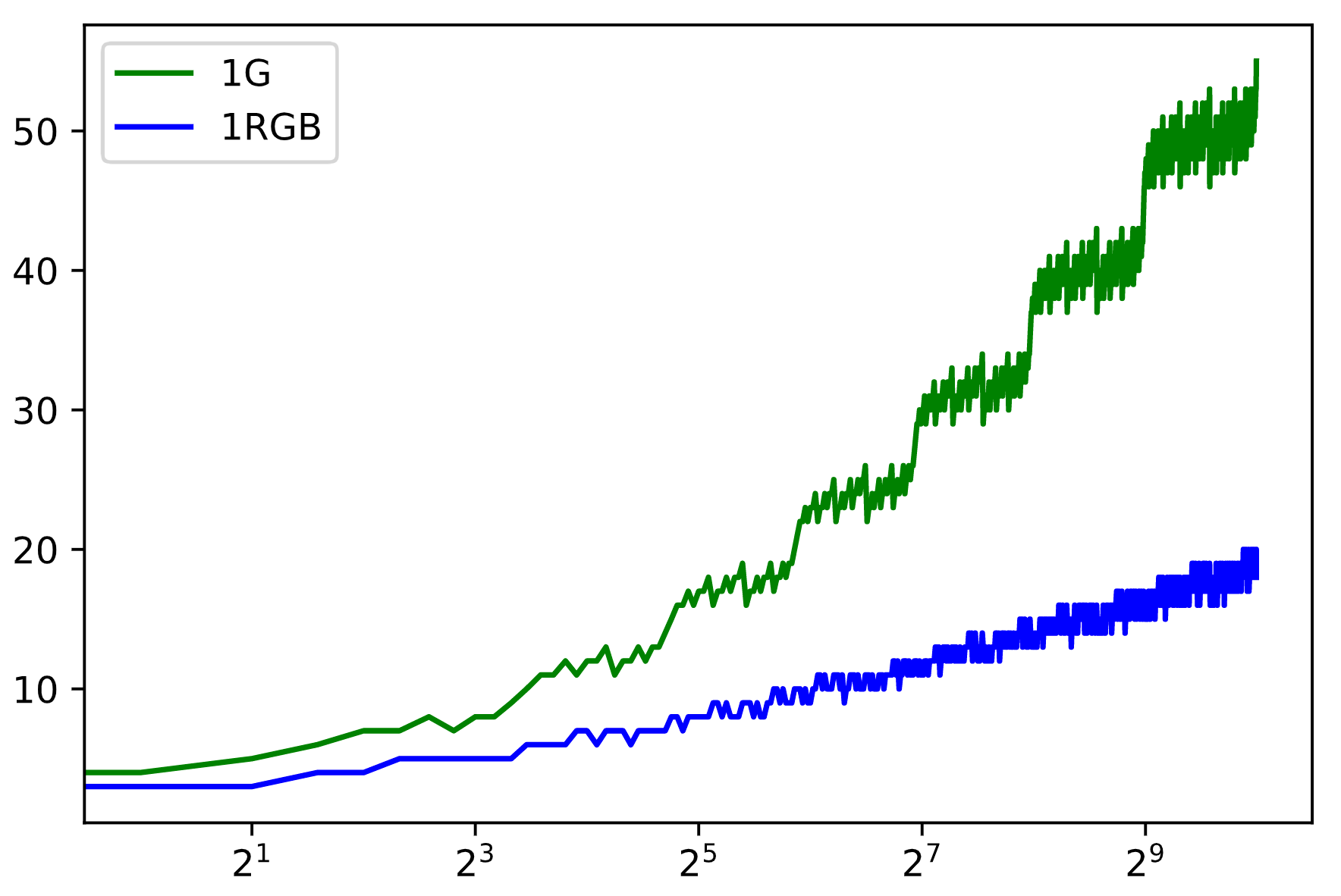
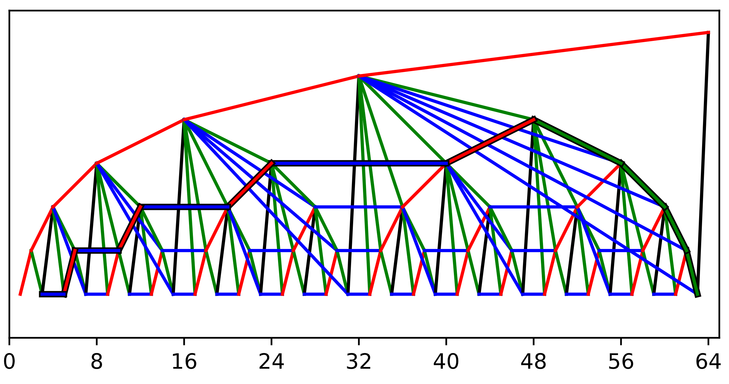
It turns out that by supplementing our “green” 2^k shorcuts with “red” 2^(k-1) and “blue” 2^(k+1) shortcuts, we can in fact accomplish log(i) indexing. This structure can be seen in the first image in this post (I’ll explain the yellow shortcuts soon). A quick experiment does seem to suggest that adding red and blue shortcuts yields log(i) indexing:
In order to understand the yellow shortcuts, it helps to use a slightly different visualization. If we raise each node in the structure to a height of k, the tree-like structure reveals itself. It’s important to remember that all of the shortcuts are still pointing from right to left, and not top to bottom as in a normal tree. This highlights the crux of what is challenging about this, and as can be seen, the path is somewhat non-trivial and has to cut awkwardly across the tree:
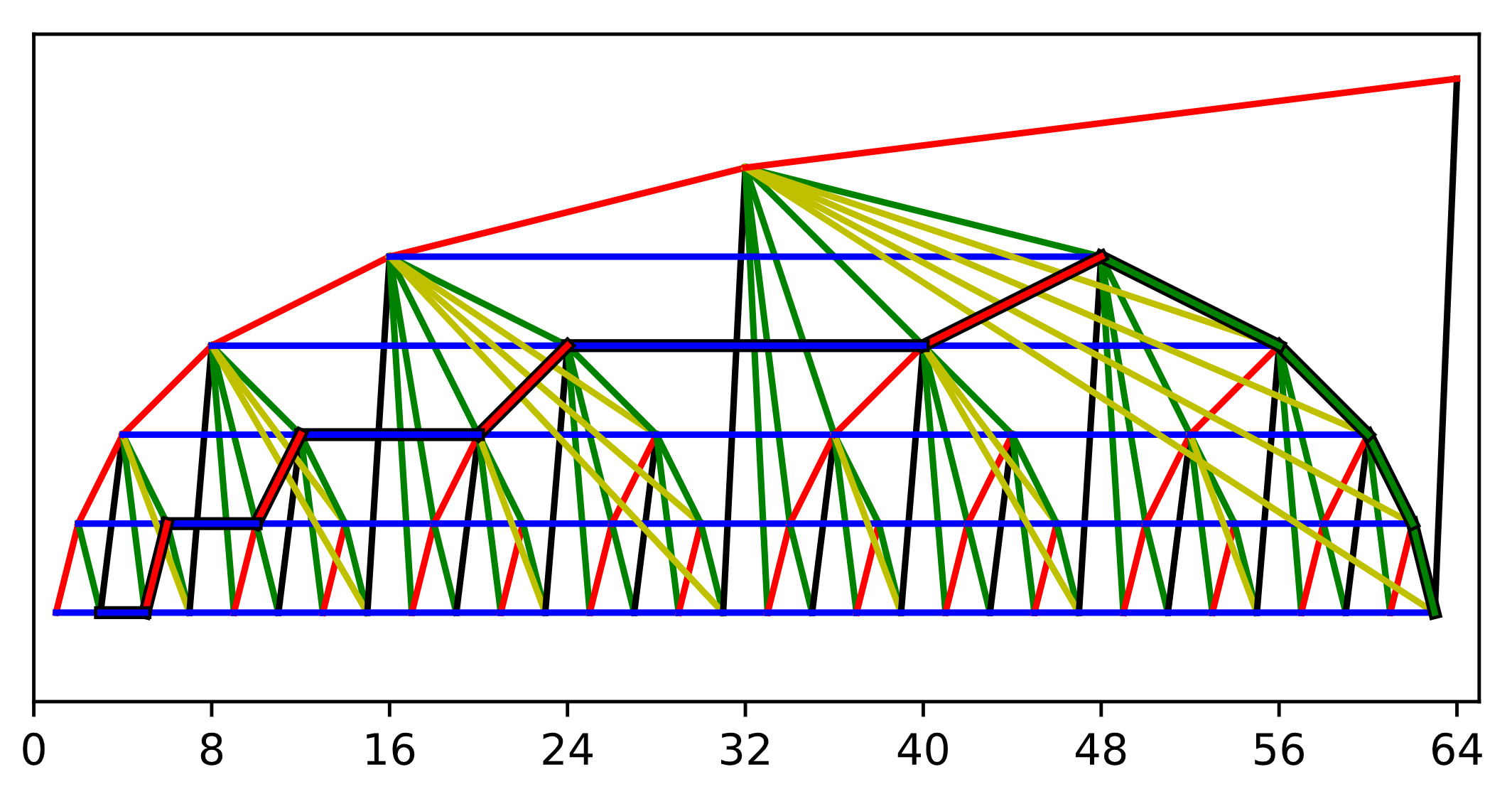
So what’s with the yellow shortcuts? They’re required in order to allow us to push/cons new nodes in constant time when building up the red, green, and blue shortcuts. Let node.n, node.r, node.g, node.b, node.y be the next, red, green, blue, and yellow fields of a node respectively. We could compute node.r as node.n.g.g…g, but this would follow log-many green shortcuts in the worst case. The yellow shortcuts are used to lazily compute this chain of greens ahead of time. Now, ignoring edge cases, we can compute the shortcuts as (each of these can be visualized as a path in the above image):
-
node.r := node.n.y
-
node.g := node.r.g
-
node.b := node.r.b.g
-
node.y := node.g.y
Now for the actual indexing algorithm itself, followed by a proof of time complexity. Each node is equipped with it’s own index as node.i. Here is the core of the algorithm, ignoring some edge cases, and an additional f function I’ll explain below:

First we convert “indexing by i” into “seeking for a specific index j”. Now, unless we’re done, we try a shortcut, preferring green over blue over red over next. This order is important and not greedy. We only take a certain shortcut if (1) it wouldn’t overshoot the target, and (2) a subsequent green hop wouldn’t overshoot a green hop from the target. The purpose of the f function is that f(i, j) recurs exactly as many times as seek(n, j) when n.i = i and is easier to reason about, so I will instead prove that f has run time logarithmic in i-j.
It is simple to verify that f always terminates with the termination metric i-j, so we don’t have to worry about over-shooting the target. I will treat G, B, R, and N as actions on an integer i and prove that any run of this algorithm has 3 phases:
-
Possibly a single N action.
-
A sequence of G and B actions, without back-to-back Bs.
-
A sequence of R and B actions, without back-to-back Bs.
Looking at the tree, one can see that this will always yield paths of length logarithmic in the distance travelled (i-j). This is because a path followed by the algorithm can only go up the tree with hops of exponentially increasing size and then back down with hops of exponentially decreasing size. Therefore it can only fit in at most logarithmically many hops. We still must prove that all paths conform to the the 3 phases, and it suffices to rule out the following action sequences: RG, RBG, BB, NN, GN, BN, RN. Each of these cases can be refuted as such:
-
RG: The algorithm would prefer a single G which is equivalent.
-
RBG: The algorithm would prefer a single B which is equivalent.
-
BB: The algorithm would prefer either GRB or BGR, depending on the bit left of the rightmost 1 in the binary representation of i.
-
NN: The algorithm always does a G from odd indices.
-
GN/BN/RN: After a G/B/R action that doesn’t get to j, we know that j<i and G(j)≤G(i). Using the universal facts that R(i)<j<i ⇒ R(i)≤G(j)<i (i.e. G arcs never cross R arcs) and G(i)=G(R(i))<R(i), it follows that j≤R(i) and G(j)≤G(R(i)). This means the algorithm always prefers an R over an N after a non-N.
Final Thoughts
There are at least a few ways in which this data structure can be improved. We can use fewer shortcuts per node: further examination of the BB case above reveals that the B shortcuts of nodes with Y shortcuts never get used, so we can drop Y shortcuts altogether and repurpose B shortcuts for those nodes. This gets us down to 3 shortcuts per node without any effect on paths. We can also optimize the indexing algorithm: since we know the algorithm ends up using 3 phases, we can explicate this to improve performance. However, my main goal with this post was simply to demonstrate that pure lists with O(log(i)) indexing can be made with relatively simple structure.
It’s worth pointing out an advantage of O(log(i)) over O(log(n)) indexing, where i is the index and n is the length of the list. Consider again the case of using such a list as an interpreter environment. With an O(log(n)) indexing implementation, the performance of a given function in the interpreted language depends on the lexical depth at which it’s defined! Similarly, consider an implementation where the nodes are blocks in a blockchain. With O(log(n)) indexing, the performance of the blockchain itself would slow down logarithmically with time.
An implementation of this algorithm in Python with a Jupyter notebook for creating the above diagrams is linked below. Note that this implementation demonstrates using bit operations in place of pointer dereferences whenever possible, which is recommended for use in imperative languages: