Transfinite Meta-Programming - Part 2
In Part 1 I attempted to give some intuition for the process of iterating reflection to infinity and beyond: any time we can iterate reflection infinitely, we can reflect on this infinite process. In this post, I’ll be formalizing this notion in a simple programming language, and I recommend reading that last post before this one. Code is linked at the bottom.
I will show how this formalization arises naturally by starting with the Lambda Calculus with De Bruijn indices and conservatively extending these indices to arbitrary ordinals. I will try to break the large language and program changes into many small changes with the hope that this will minimize the amount of explanation required.
Since we are dealing with meta-programming and quotes, it is important to distinguish concepts within the language from those outside of it. I will use markdown code blocks to name terms of the language from the outside. I will call the language used to implement the full language the "implementation language". I used Scala as the implementation language, but this should be irrelevant for this post. Also note that while I resort to operational nomenclature to help convey concepts, the language presented here (and its implementation) are purely functional.
De Bruijn Indices
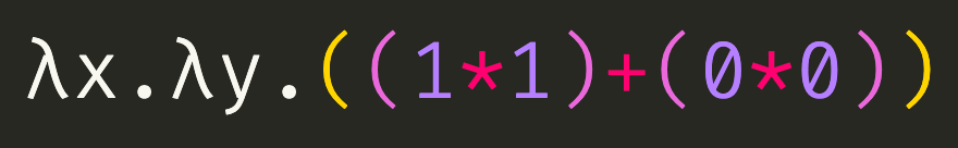
We start with simple Lambda Calculus extended with some basic arithmetic operations. Here’s a program that takes two arguments named x and y, and returns the sum of their squares:

The above program specifies a function that when applied to 3 and 4 returns 25. But that’s a lot of parentheses, but with an improved parser we can equivalently write:

The above program contains two lambda terms: λy.(x*x)+(y*y) and λx.λy.(x*x)+(y*y). Any point within a program is inside some sequence of lambda terms, from innermost to outermost. At all variables in the above program, the sequence of lambda terms is [λy.(x*x)+(y*y), x.λy.(x*x)+(y*y)]. Taking the variables bound by these lambda terms gives the sequence [y, x]. We might say that some point in the code "sees" that sequence of variables when looking outwards.
Now we will introduce De Bruijn indices. We can replace each variable in the above program with it’s index in the sequence of variables that it "sees". These are called De Bruijn indices:
The 1 indices refer to x and the 0 indices refer to y, based on the [y, x] sequence they both see. The 0-indexing is important here. But of course, this is confusing. The indices look like integer values, so the whole program looks like it takes two arguments but always returns 1. Let’s instead write:

This looks needlessly verbose, but it will be consistent with what we’ll need soon. The real language provides nicer syntax for writing the same thing, but if I used that now things would get confusing.
Notice that the variable names are no longer used, so we can just write:

Let’s think a bit about how an interpreter might process the above programs. Loosely, the interpreter is a recursive function that walks the syntactic representation of the program, adding, multiplying, and applying when needed. In order to look up the passed value of a variable like [,1]v, it needs to keep track of which actual values were passed to each of the lambda terms that it sees. It does this in a data structure called an environment. For example, if the above program were applied to 3 and 4, then at the [,n]v terms, the interpreter would have the environment [4, 3]. Notice that the order is reversed from how the values are passed in. Now the [,1]v simply resolves to the 1st value from the environment: 3. Note the correspondence to the more direct understanding when we used named variables.
Splices
Operationally, when the interpreter sees [,n]v, it chops n values off the front of the environment, and then returns the first value of the resulting environment. Let’s split this into two separate things. The [,n]t will be called a splice and will tell the interpreter to descend into the body t with an environment chopped by n. The v will simply pop the first value off the environment. Now we can rewrite the above like:

A chop by 0 doesn’t do anything, so those have been removed. In fact, the actual language doesn’t even allow such no-ops. Now that we can attach splices to terms other than v, we can simplify further to:

Note that the vs look the same but return different values because they are interpreted in different contexts (with different environments). Also note that we’ve avoided the duplicate work of chopping the environment twice by combining both splices.
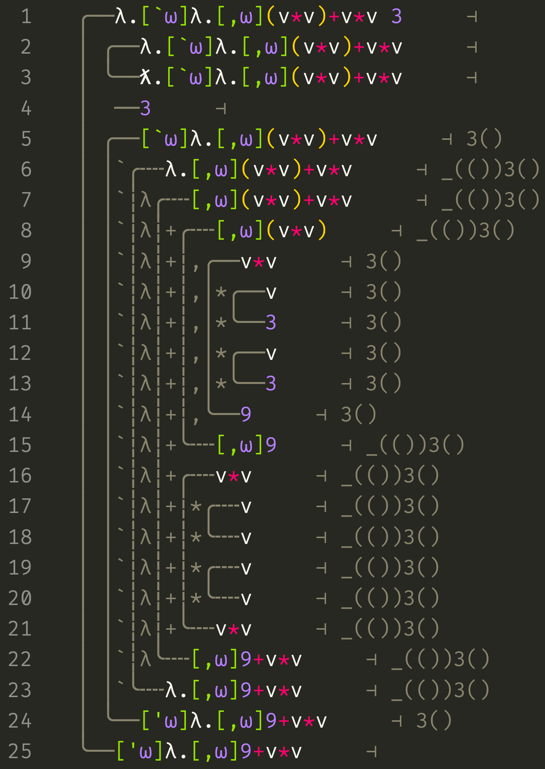
Before we continue, we should take a look at how the interpreter handles this:

This is a trace of an execution of the interpreter on the program above applied to 3 and 4. The pipes on the left connect terms at the top to their resolved values at the bottom. Their nesting shows how the interpreter descends into terms. Symbols to the right of a pipe hint at the kind of term at the top and help our eyes follow a given pipe downwards. The right side of each line depicts the environment at that term. The ƛ terms are called closures; they’re λ terms but with an environment attached. Note how the outermost term is processed by first processing the outer lambda term, then processing the 4, and then processing the body of the lambda term in an environment containing 4. I won’t delve on this any further here.
Most importantly, note how [,1](v*v) is processed in the environment [4, 3]. It chops one value off the environment to yield [3] and then processes v*v in that environment. If you’re surprised that this term resolves to 9 rather than [,1]9, hold on to this concern because it will be important later.
Transfinite De Bruijn Indices
From this vantage point, our big mental leap to meta-programming becomes a small one. We can "simply" extend the domain of our De Bruijn indices to transfinite ordinals. There are some tricky details, but we can get started rather easily. Let’s just try it and see what breaks:

The error handling in this language could certainly be improved, but it’s hopefully clear what went wrong: by splicing by ω, we chopped off the entire environment so that when v tried to pop the value off the front, there was nothing there. We can fix this by introducing a new kind of term:
There’s a lot of new stuff here and our input program is a little buggy, but let’s focus on the evaluation of the [`ω]t term which starts at line 5. If we follow the pipe down, we can see that it resolves to a [‘ω]t value called a quote representing a piece of code. The original term is called a quasiquote and is used to build such quote values.
Inside the evaluation of this term a couple things change. The environment annotation contains a (()) before the 3 value. If you’ve read my other posts, you might recognize this as a representation of the index ω by which we’ve quasiquoted. This is because an environment is simply a function from ordinals to values, i.e. a transfinite list. The effect that this has is to put the value 3 beyond infinity in the environment. No normal (finite) De Bruijn index could reach it from inside the quasiquote, because the value exists at the meta-level.
In order to reach the value 3 in the environment, we need an infinite splice, like the [,ω](../../v%2Av) term on line 8. Stepping into this term chops the (()) gap off the environment, so that the v*v on line 9 may resolve to 9. It is important to note that this is not a new language feature; this splice behaves exactly like the splices in the earlier examples. All we’ve done is extend the set of legal indices (and the domain of environment maps) to infinity and beyond.
Now note the difference in behviour of the v*v term on line 16: it resolves to itself. This is strange because it isn’t a value, but context is everything. Whenever the environment contains an infinite gap and so has infinte length, we’re inside a quote and the interpreter behaves differently. The interpreter will build code terms rather than values. In particular, variables won’t be resolved and operators like * will build terms from their arguments. The traces make this extra apparent by making the pipes dashed.
Lift and Run
The above code was demonstrative but not quite correct. We’d like it to build a specialized lambda functions that map values y to 3*3+y*y that has been constant folded, i.e. λ.9+v*v. We can accomplish this with the 2 remaining staging operators (parts of this trace have been removed for brevity):

The [^ω] term on line 10 is a "lift" operator. It evaluates its body with the environment unchanged and then lifts the resulting value to a quote with the specified index. In this case, that resulting quote is spliced into the surrounding quote of a lambda on line 20 which contains the term we were trying to build. Finally, we need to "run" this quote with a [%ω] operator to yield a closure which in this example is applied to 4.
To summarize the 4 staging operators, excluding quotes which are values:
-
[`n]tis a quasiquote. It evaluatestin the environment padded bynto yield a quote. -
[,n]tis a splice. It evaluatestin the environment chopped bynand splices the resulting quote into the surrounding quote. -
[^n]tis a lift. It evaluatestin the current environment and then builds a quote. -
[%n]tis a run. It evaluatestin the current environment, unwraps the resulting quote, and evaluates the resulting term.
Implementation
The implementation of the language isn’t so different than that for our original lambda calculus but with extra operators for staging, simple ordinal arithmetic, and some tricky cases to be careful about. I’ll detail a few of them here.
As mentioned above, empty splices like [,0]t are disallowed by the language. More generally, the language implementation insists on keeping all terms during computation in a normal form with respect to these staging operators. This normal form excludes terms like [,a][,b]t in favor of [,c]t where c is equal to a plus b. For example, [,ω][,1]t is avoided in favor of [,(ω+1)]t which splices up 1 meta-level and then 1 normal De Bruijn index. On the other hand, [,1][,ω]t is avoided in favor of [,ω]t. Intuitively, splicing by 1 (or any finite) De Bruijn index is irrelevant when followed by a splice to a meta-level. This shows that splices don’t necessarily commute.
Not all staging operators combine the way that splices do. To see (one reason) why, let’s look at a trace with a "big" quote:
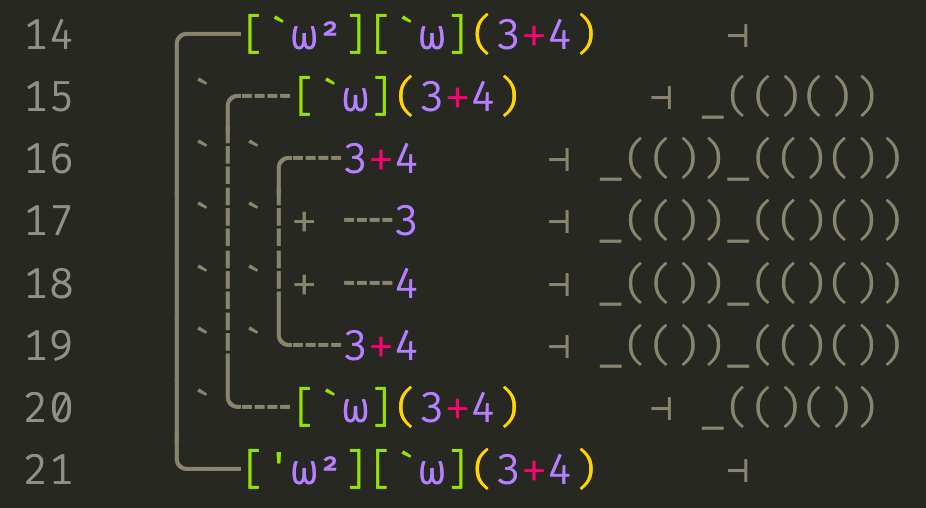
The result is the funky looking [‘ω²][`ω](3+4), a quote containing a quasiquote. Not only was the addition not resolved, but the inner small quote wasn’t either: it remained a quasiquote. The way to think about this is that the ω² dominates the ω, treating it like a value within the body of its quasiquote. I’ll define domination in a second, but it basically just means one quote is much bigger than the other. A simple reason why we can’t use [`(ω²+ω)](../../3%2B4) above is that it might resolve to [‘(ω²+ω)](../../3%2B4), which is incorrect.
There are a few equivalent ways to define when an ordinal a dominates b:
-
a >> bwhenb+a = a -
a >> bwhena > banda+b != b+a(aandbdon’t commute additively) -
a >> bwhenb = 0ora = ω^c+dandb = ω^e+fandc > e(ahas a bigger exponent thanb)
What this implies is that quasiquote indices must be of the form [`ω^x*y] for some ordinals x and y, otherwise they’re the result of combining an ordinal with another that it dominates. That is to say, they must be monomials, or multiples of ω. This restriction suggests another representation of non-finite quotes: as quotes of a certain bigness (x) repeated a certain number of times (y). In the case of multi-stage programming, x is always 1, and in the case of simple meta-programming, y is also always 1. In fact, one could introduce multiple incomparable "flavors" or ω representing different languages in a non-total order of indices and transfinite splices would still make sense, but I’m getting ahead of myself.
Examples and Higher Stages
I’d like to build towards the unstaging example I shared in the last post. Let’s start with a simple exponentiation function (with most of the trace removed again):

The only new feature here is the f. It works exactly like the v but instead of popping a passed argument off the environment, it pops off the function to which that argument was passed. In the trace above, the f pops off the inner lambda term that accepted the exponent argument so that we may recurse on it.
Now let’s stage this program to yield a code generating function. I’ll simplify the syntax a bit to use ` and ‘ and , as shorthand for [`ω] and [‘ω] and [,ω] because ω indices are very common. I’ll also use v1 in place of [,1]v to make normal De Bruijn indices less verbose.

The first thing to note is that we are in fact returning a quote of a term which would resolve to 8 and delaying the actual multiplication to resolve it. The result could of course be run with a %. The next thing to notice is that instead of just passing the number 2 to the function, we’ve passed a quoted 2. This is fairly natural because the code of 2 appears in the output at the same "level". On the other hand, the 3 gets used as a number rather than code so is passed unquoted. The final thing to notice is that this program is exactly the same as the one above except with staging operators inserted. Our final example will be a program to undo what we just manually did and remove these operators, but we’re not ready yet.
Instead of passing a quoted 2, we can pass a quoted v and add some boilerplate:

This builds residual code which cubes its inputs. If we’d passed a number other than 3, we’d get residual code for other powers. If we’d staged a more efficient exponentiaion function such as one that used iterated squaring, we’d get more efficient residual code like λ.(sqr (sqr v)) for powers of 4. We could have fun here and this is all well explored, but let’s go higher.
In order to effectively work with code objects in a functional language, it is helpful to have pattern matching tools. To this end, let’s generalize lambda terms to pattern lambdas which pattern match on their inputs:

The term to the left of the . is the pattern and the term to the right is the body as in a normal lambda. Applying a pattern lambda to an argument starts by inferring an environment in which the pattern would evaluate to the argument. For example, above the environment ‘3()’4() is inferred because in this environment, the pattern `(,v+,v1) evaluates to the argument ‘(3+4). After this sort of backwards evaluation, normal forward evaluation takes place on the body in this inferred environment. The v1 and v are swapped in this pattern lambda, so the result is that the 3 and 4 are swapped in the output. To write a normal lambda as a pattern lambda, simply use v as the pattern.
Each pattern lambda is a term rewriting rule, but we’ll need a way to combine them. First an example with some syntactic sugar:

We’re using some new library assignment syntax to make authoring programs a little less painful, which hopefully doesn’t need explanation. The | is syntactic sugar which has the effect of combining pattern lambdas. The first pattern lambda works on addition terms, while the second works on multiplication terms. I’ve decided to make pattern lambda application evaluate to 0 when the pattern doesn’t match the argument. Now for the trace:
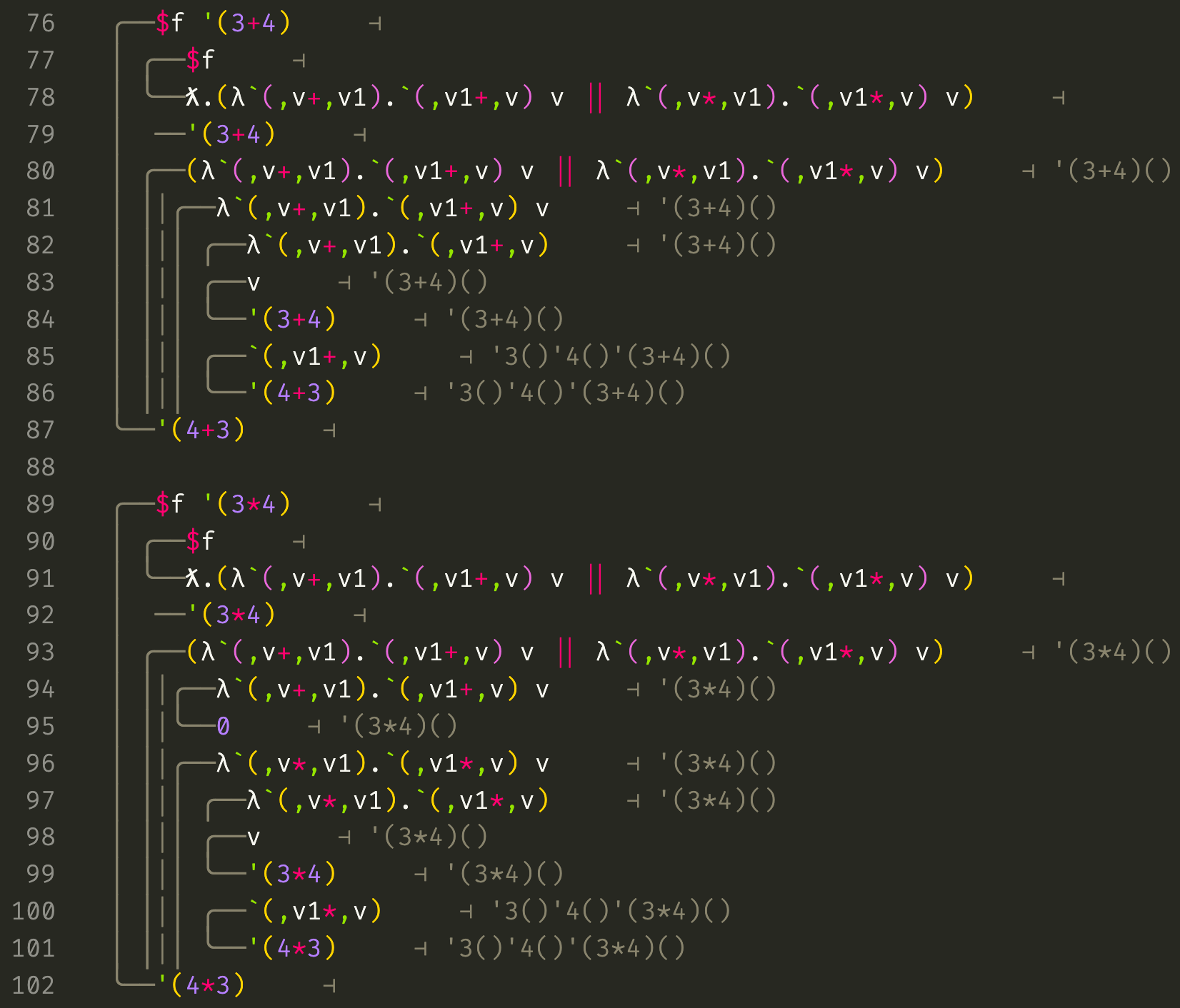
We can see on line 78 what the syntactic sugar f|g expands to: λ.(f v) || (g v). The || operator is the usual short-circuiting boolean "or". This will first try (f v) and if that fails to match and returns 0, it will try (g v). The trace shows that this can be used to build a function that can handle multiple types of inputs.
Now at long last we can write our first transfinite meta-program, $unstage:
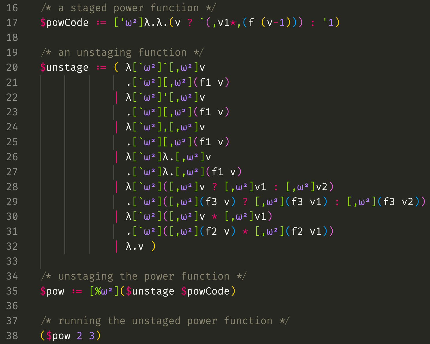
The input $powCode is the big source code for the staged power function above. Having access to a program doesn’t imply having access to it’s source code (!(x → r)), so we must explicitly provide it’s source code at the ω² level so that $unstage which lives there may inspect and rewrite it. All of the pattern lambda cases withing $unstage (except the last) recurse structurally on the subterms of the input by calls to f1, f2, or f3. These all refer to $unstage but are at different depths because of the differing number of pattern variables in each pattern. The last catch-all case is the identity function and simply returns the term without recurring if nothing else matches. Note that the first few pattern cases are able to safely talk about small staging operators without interacting with them by using "big" quasiquotes, which was our goal from the start. The full trace can be found here: Trace
Conclusions
The programming language I’ve presented is still in a few senses unsatisfactory. There is nothing in place to guarantee that the programs we generate are legal and have no unbound variables. The operators and quote values are in a sense very "raw" in the sense of an assembly language and require us to manually take care of our variables, lambdas, and indices. An improvement upon this language might try to automatically manage these things, perhaps by storing index "shifts" within the environment.
The traces built are in some cases unnecessarily long because quotes are walked multiple redundant times. It may be possible to solve this by unifying quasiquote with quote into a single term variant with two parameters: size and "valueness". However, this makes it difficult in the implementation language to distinguish values from unresolved terms without fancy/dependent types.
That being said, I’m happy with this little language. Scary glimpses into the depths of reflection upon reflection upon reflection have kept me awake at night, and I feel that even if this language is complete bogus, I have some sort of framework for addressing such "recurring thoughts".
Finally, I should give credit to the paper "Multi-stage programming with generative and analytical macros" against which I tested the initial MSP fragment of this language and from which I borrowed some examples. The author Nicolas Stucki also answered several of my questions and taught me some Scala.
The code can be found here: https://github.com/asvarga/Transfinite-Meta-Programming